Converting Clutch into Wins - A Pythagorean Model for Tennis
In the short life of this blog, I have, on several occasions, complained about the lack of analytics in tennis. But what evidence is there to back up this view? One place to start to unpack the state of analytics in tennis is by comparison to other major sports that are at the forefront of the analytics revolution. In this article I want to discuss one gap that such a comparison reveals— the lack of metrics for win expectation.

Win prediction is often referred to as the “holy grail” in sports statistics. This was one of the first problems tackled by Bill James, the father of sabermetrics and catalyst of the Moneyball sea change in baseball. A major contribution James made earlier in his career was to derive a simple formula to calculate a team’s season win expectations based on a single measure of strength: runs scored. James presented his formula in the 1981 Baseball Abstract. Sadly, I couldn’t find an electronic version of that piece so I will reproduce the formula here:
$$ \mbox{Win%} = \frac{RS^2}{(RS^2 + RA^2)} $$
Here, $RS$ are a team’s runs scored in a season, summed over all games, and $RA$ is the corresponding runs allowed, that is, the sum of runs their opponents earned against them in the same games. Because of the similarity of its form with the Pythagorean theorem, it has become known as the Pythagorean expectation for wins.
Since its discovery, versions of the Pythagorean formula have appeared in most major sports. Perhaps the most famous version is used in Ken Pomeroy’s NCAA basketball ratings, which have become the go-to resource for predicting brackets for the March Madness tournament.
But, to my knowledge, no application of the Pythagorean formula exists for an individual sport. At today’s New England Symposium on Statistics in Sports (NESSIS), I wanted to change that.
In a talk presented at NESSIS, I extend the Pythagorean formula to tennis. The main question this work wanted to answer was whether there is a simple performance measure in tennis that approximates the Pythagorean relationship and is also an accurate measure of a player’s match wins in a season? The surprising punchline is yes.
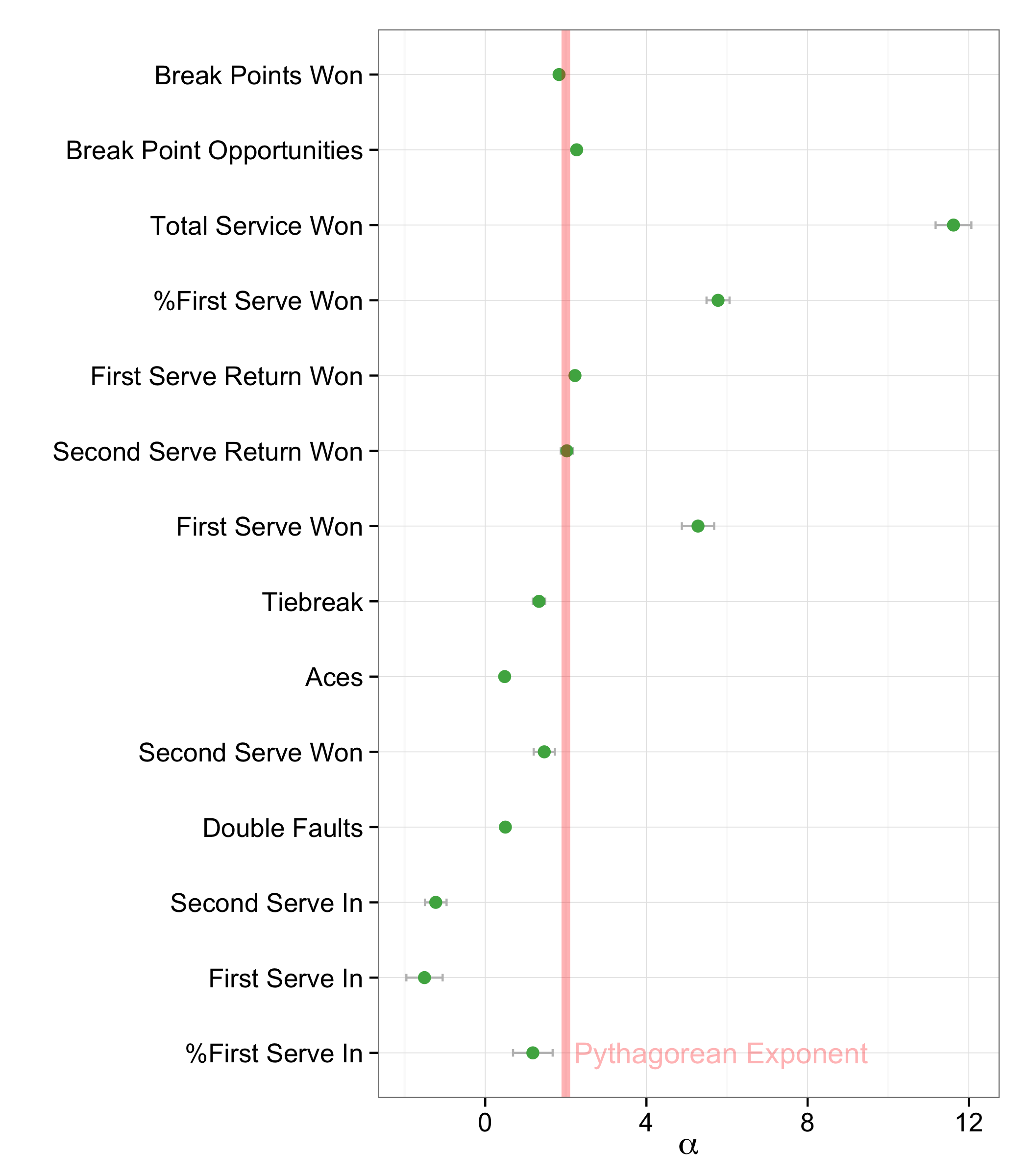
When 14 common performance measures were plugged into the following general form of the Pythagorean model, using ATP match data for 2004 to 2014 (over 50,000 matches),
$$ \mbox{Win%} = \frac{X^\alpha}{(X^\alpha + Y^\alpha)} $$
several were found to give a coefficient close to the Pythagorean coefficient of 2. Interestingly, all relate to return performance: break points won, break point opportunities, first and second return points won. (Note that some measures, like total return points won, are not considered here because they were very highly correlated with one or more of the other measures considered.)
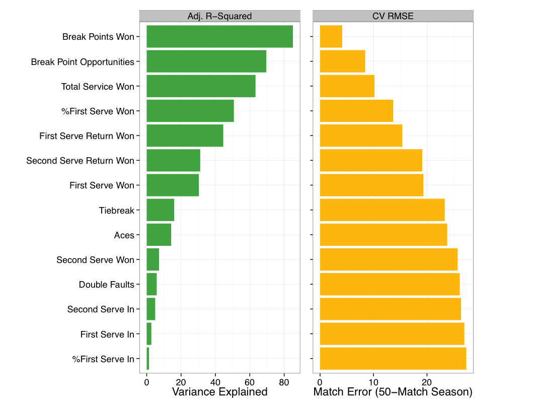
More importantly than the coefficient of the fit is the model performance. The fit of each of the possible Pythagorean models are shown in Figure 2 based on adjusted R-squared and leave-one-out cross-validated error. An R-squared of 100% is the best fit possible as it indicates that the model explains 100% of variation in match wins. The cross-validation error summarizes the deviation in predictions from what is observed in a way that is more robust to training-data bias. What both of these measures show is that the Pythagorean model based on break points won is without question the best-performing model of the group— explaining 85% of variation in a player’s season match wins with the lowest error.
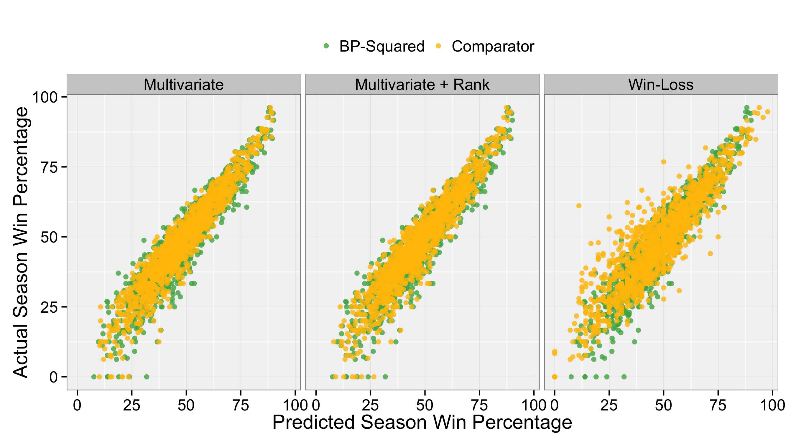
This looks impressive but maybe the break point model, what I will call $BP^2$, looks good because it is being compared to models that are all collectively poor. As a better test of the performance $BP^2$ I compared its season-end projections based on mid-season break point strength for the 2004-14 seasons against the corresponding $Win%$ projections for three alternatives: win-loss record, a multivariate model that included 11 of the 14 measures (including break points won), and the same multivariate model that included player’s relative rank.
The scatterplots in Figure 3 show the results. Interestingly, win-loss is the worst, as is indicated by the greater cloud of points around the line, i.e. more deviations from the linear relationship. The projections for the multivariate model without rank is the best, presumably because some of the arbitrariness in ranking point assignments and player schedule selections adds noise to the version of the model with player ranking. But $BP^2$ is very comparable to the multivariate model, both yielding a 50-match season error of $\pm$2 matches.
So, this brings us to the perhaps obvious conclusion that break point conversion is important for winning in tennis. However, this isn’t the innovation here. The innovation is that $BP^2$ gives a formula to quantify exactly how important break point conversion is and reveals an eerily similar relationship as the one originally proposed by James between runs and wins in baseball.
Some Implications: Clutch Charts
The discovery of $BP^2$ has a number of potential implications for prediction and performance evaluation, too many to give enough attention here. But I did want to suggest one direction of work that could use $BP^2$ to improve our understanding of outcomes in tennis.
There has been a lot of discussion about Federer’s break point performance contributed to not bringing home the US Open trophy this year. Using a 9-month look back, the chart below shows the timeline of Federer’s win expectations in 2015 and how it related to each win and loss.
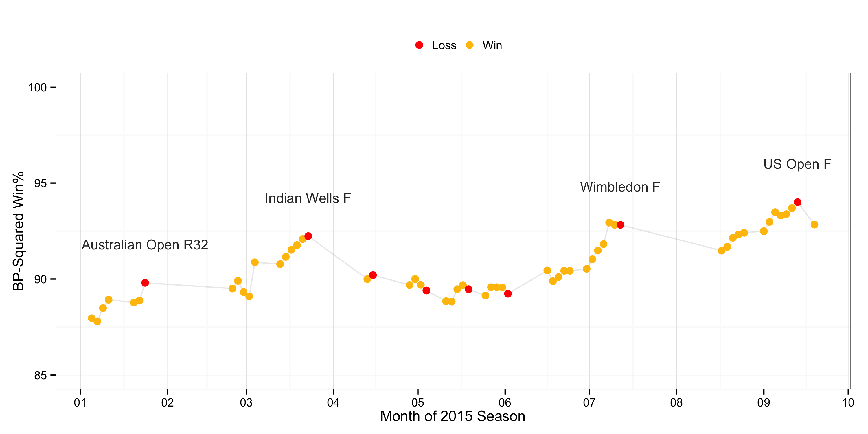
There are a number of insights this chart reveals. Outside of the clay court season, Federer’s big losses were generally preceded by a rise in break point strength and a subsequent fall. Note that each point is the win expectation going into a match so the drop following a match tells us that break point conversion was very likely a strong contributing factor. The rise-and-fall pattern also tells us that he entered the finals of several major tournaments (and two majors) with an accelerating win expectation but didn’t play to expectation in the final. This was particularly dramatic at Wimbledon.
Of course, a loss ultimately is a function of a player’s win expectation relative to his opponent’s, but the chart of Federer’s individual $BP^2$ strength does corrobarate the general impression, and Federer’s own impression, that clutch performance was what made the difference for his losses at the Grand Slams. It also shows that he had a spectacular season, major win or not.