What a Model of Player Availability Can Tell Us About Probable Injuries in Tennis
The 2020 tennis calendar was put into a tailspin by the pandemic. In a normal year, a player’s competitive schedule can tell us a lot about a player’s overall readiness to play, what I will call a player’s ‘availability’. In this post, I show how a Hidden Markov Model can be used to describe a player’s competitive schedule as the output from periods of varying availability and how irregularities in availability can be a tell-tale sign of probable injury.
The concept of player availability is a common one in team sports, where ‘available’ players are the ones who are fit and ready to compete if the coach chooses to put them on the starting lineup. This means that the observation of a player in competition, compared to a player on the bench or on an injury list, is telling us something about that player’s fitness.
Now, there are no rosters in tennis. But a player still has to be available to compete. And, like elite athletes in team sports, tennis players want to compete wherever they think they have a chance to win against strong opponents. So when they skip big opportunities, it is reasonable to suspect that something out-of-the ordinary is going on.
We can see this with even a handful of playing schedules for top players. The chart below shows the weeks, out of the 46 weeks of the usual calendar, 30 of the top male players competed in 2019 (what feels like a bygone era now). For players that are eligible to compete in any week they like, we see that most are competing in 25 weeks or more, in other words, more than 55% of the time.
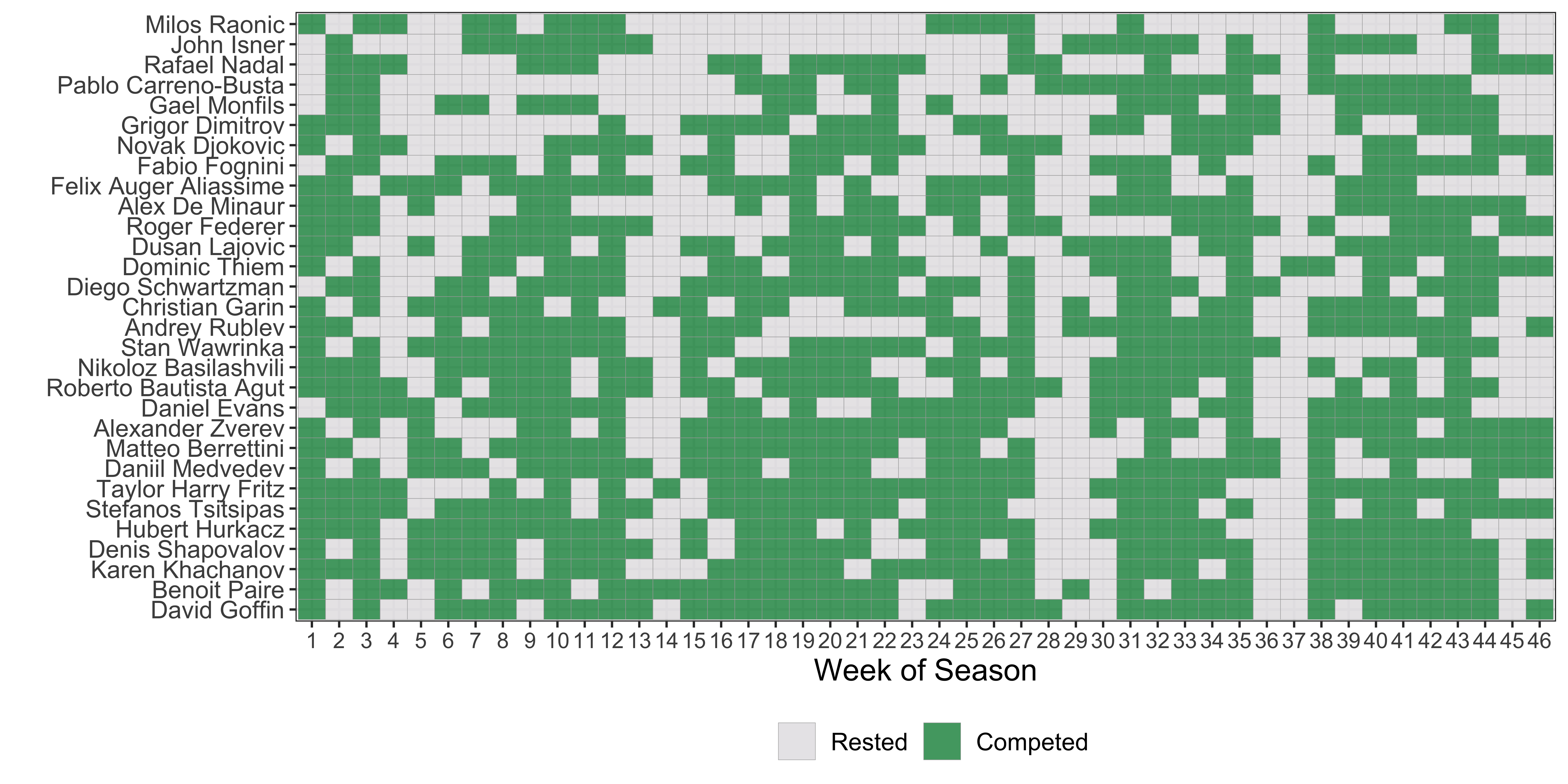
But we can also see a few players who didn’t follow this pattern. In fact, I’ve sorted the schedules from top to bottom in terms of the fewest competition weeks played. Big men Milos Raonic and John Isner were out of commission for extended periods in 2019. Rafael Nadal and Pablo Carreno Busta also had some surprising long absences from competition.
If we wanted to know when a player had an unexpected absence from competition and what the cause might have been, we could comb through wiki pages and media reports and hope that someone out there was tracking the ins and outs of that player’s scheduling decisions. But what if we wanted something more automatic? What if we wanted a more reliable way to detect periods of unusual gaps from competition that we could use for every top player?
The sample of timelines from above tell us that a regular patterns should be easy to quantify. We just need a reasonable model to describe those patterns and a large enough sample of schedules to apply that model to.
The first part of the model is the description of the underlying available states a player is in for any given week of the calendar (weeks 1 to 46 will be the model’s time scale). A simple but reasonable starting point is to think of a player as being in one of two possible states at any time: available or not available. The available state would be when a player is fit and rested enough to compete that they are more likely than not to enter a tournament in a given week. The ‘not available’ state is the opposite of this; which could include injury, suspension, or other personal reasons that would keep a player out of competition.
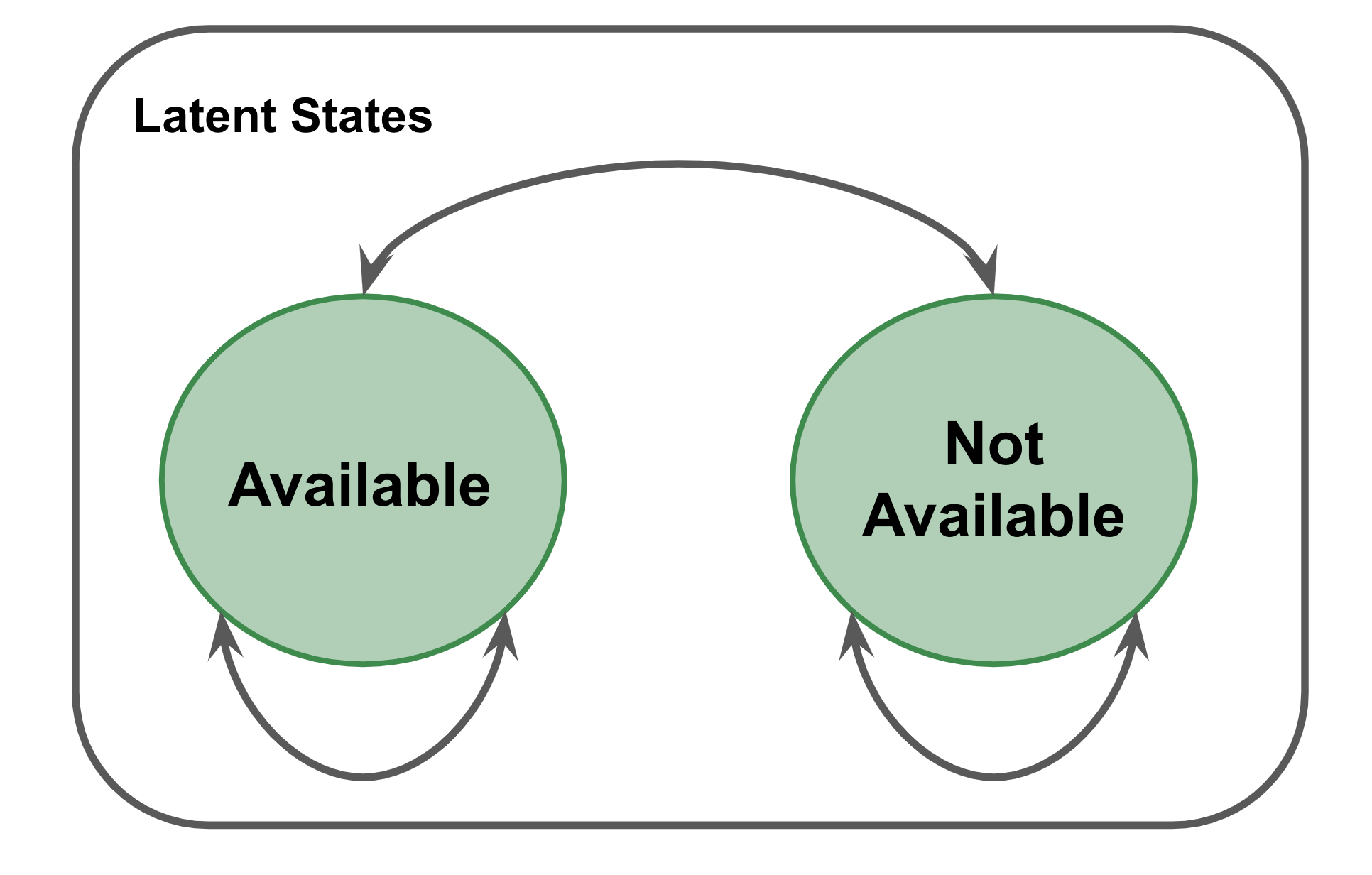
Clearly the ‘not available’ isn’t very specific. And we can imagine breaking this out into more of the cause-specific states that would result in an unexpected absence. However, we need information to differentiate among them because we are assuming that these states can’t be consistently observed. These are hidden ‘latent states’ that we will use the sequence of competition and rest weeks to infer. And from that data alone, we would have no way of differentiating a break due to a drug suspension say or a break due to a serious injury. So we will stick with the broad ‘not available’ option.
How is a player’s available state in any week determined?
Those moves are defined by a first-order Markov chain. Let’s use $t$ to indicate the week in any given season and let $a_t$ be a player’s available state $\lbrace 1 = available, 2 = not available \rbrace$. A player’s initial state is a coin toss defined by the probability vector $\boldsymbol{\pi}$,
$$ a_1 \sim Categorical(\boldsymbol{\pi}) $$
And all subsequent transitions are coin tosses from a probability vector that is defined by the previous latent state. Thus, the Markov chain in an HMM is only concerned with the most recent state,
$$ a_{t + 1} \sim Categorical(\boldsymbol{\alpha}_{a_t}) $$
Each $\boldsymbol{\alpha}_a$ is a row in a transition matrix, which, after the initial state, fully describes the latent availability model,
But what about the actual data? So far everything we’ve discussed has only been about the states we can’t see. How does the competition data fit in? To answer that, we need the final piece of the model: the observation model.
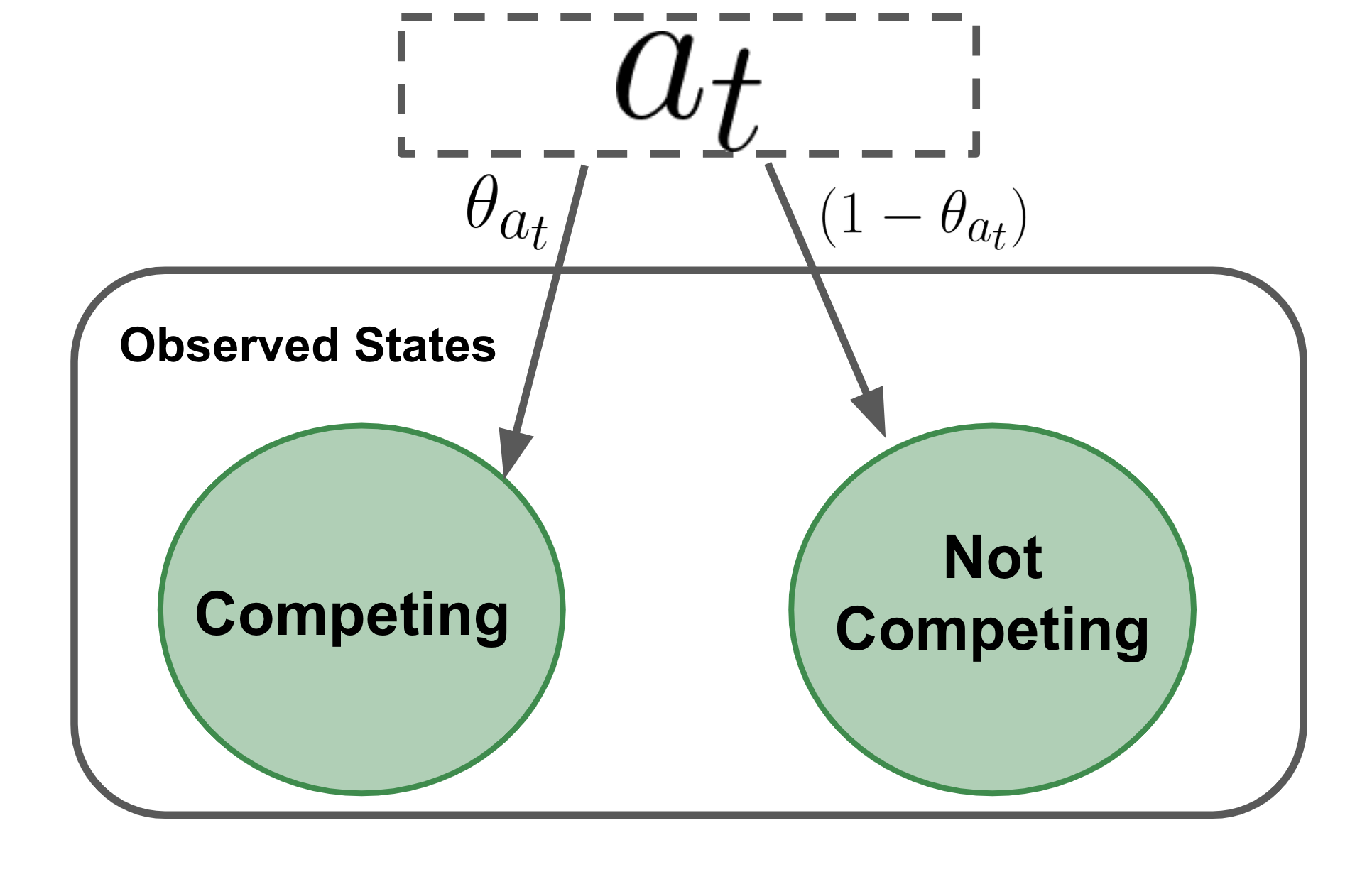
The figure to the left is a visual summary of the observation model. There are two possible observed states in each competition week—a player is either in competition or not. And the probability of being in competition, $\theta$, is determined by which availability state a player is in that week. So the observational model is conditional on the unknown latent state.
The observed outcome is a discrete event, like the availability states. This means that the draws describing the observation model have a very similar look to our latent state model. Specifically, the competition state $y_t$ is a coin toss that is dependent on the success probability $\theta_{a_t}$,
$$ y_t | a_t \sim Bernoulli(\theta_{a_t}) $$
Although HMMs can be fit with frequentist methods, a Bayesian model provides a number of advantage. First, languages for Bayesian inference, like stan, are low-level enough that we can build in a wide range of complexity for non-standard problems. Second, incorporating constraints on parameters, is quite straightforward and this can be crucial to avoid identifiability problems with latent variable models.
Let’s take our $\theta$ parameters for the availability HMM. These are the probabilities of competing in a given week: one when a player is available, $\theta_1$, and the other when he is not, $\theta_2$. Both are on the probability scale. But with no more information to distinguish one from the other, there would be no way to ensure that $\theta_1$ corresponds to the available state and vice versa.
So we need to build in some more prior information. Now, if we think about a healthy tennis player, whose income and ranking both depend on competing regularly and going deep into events wherever possible, it would be reasonable to assume that he will be competing more than not during the tennis season. This would suggest constraining the probability of competing when available to be greater than 50%. When injured or otherwise not available, the opposite would be a reasonable expectation.
A simple way to enforce these constraints is with a bounded inverse logit. The way this works is to sample a standard normal variable, $\tilde{\theta}_1$ and then set $\theta_1$ equal to,
$$ \theta_1 = 0.5 + 0.5\mbox{logit}^{-1}(\tilde{\theta}_1) $$
Whereas for $\theta_2$, we would constrain it to be between (0, 0.5) with the following,
$$ \theta_2 = 0.5 \mbox{logit}^{-1}(\tilde{\theta}_2) $$
The other hyperparameters will be given non-informative Dirichlet priors. The full stan model is given at the end of the post and makes use of new HMM functions. There is hmm_marginal to calculate the marginalized log-likelihood and hmm_latent_rng to sample the latent states given an observed sequence of competition weeks.
I fit the availability model for the competition schedules of the 30 players shown in Fig. 1 for years 2015 to 2019. Only ATP and Grand Slam events were considered. Any seasons where a player was under 18, and could still be competing on the junior circuit, were dropped.
The first set of results we consider are the posterior means for the availability transition matrix (Fig. 2). Unsurprisingly, both states are sticky. This means that a player that is either available or not will tend to stay in that state for longer than a single week. In fact, we can estimate the expected duration of each available state pretty with a standard HMM because the time to a change is a geometric distribution with probability $1 - \alpha_{a_t}$. For the available state, this would imply an expected period of availability of 50 weeks, or more than a full season of availability for most players.
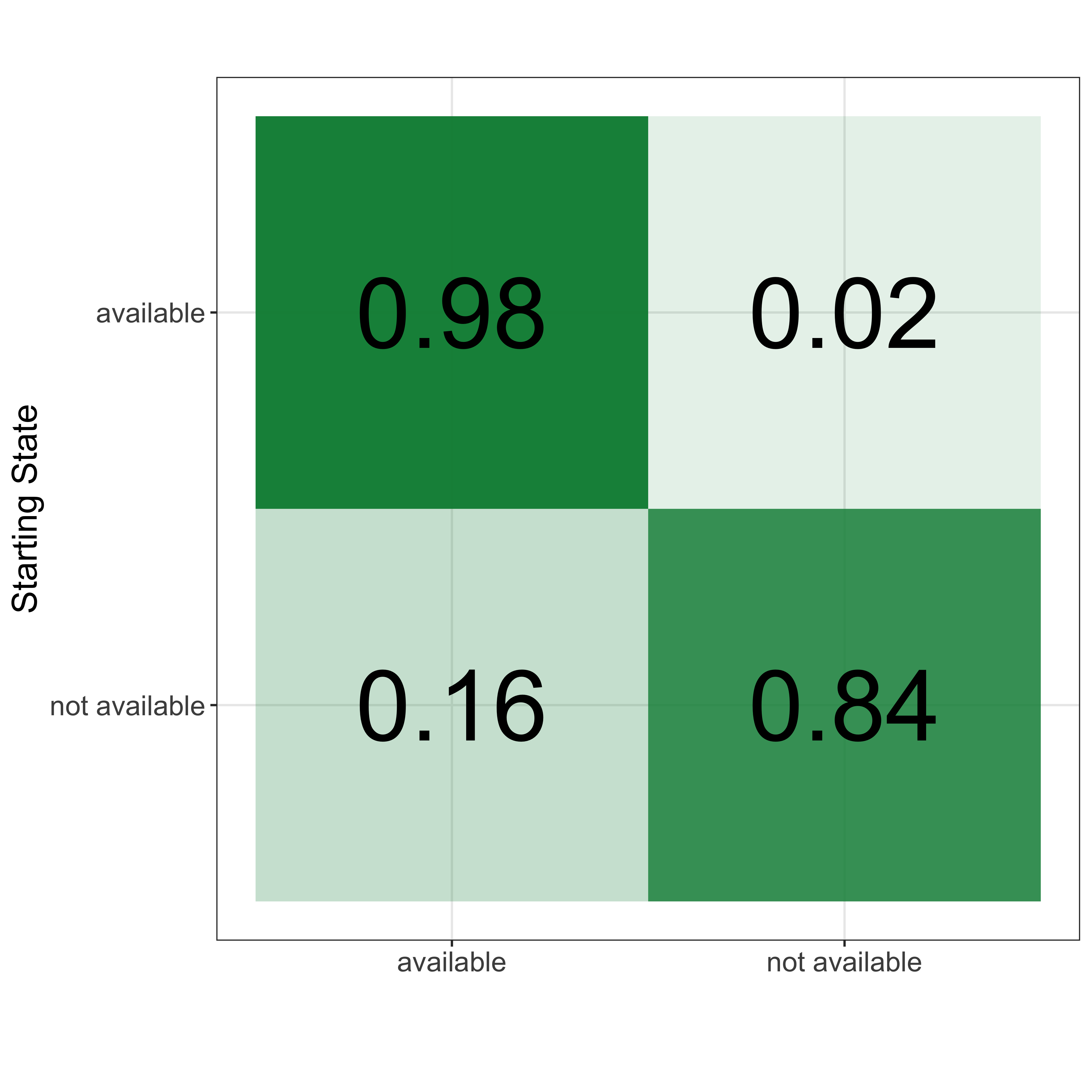
For a time-independent HMM, the transition matrix has a steady state and we can find that by raising the transition matrix to a high power. This is like going through many, many competition weeks and possible transitions. The steady state is useful because it tells us how often we would expect a random top player to be available or not available at any time during a season. From the transition matrix for this sample, we find that players are not available 10% of the time.
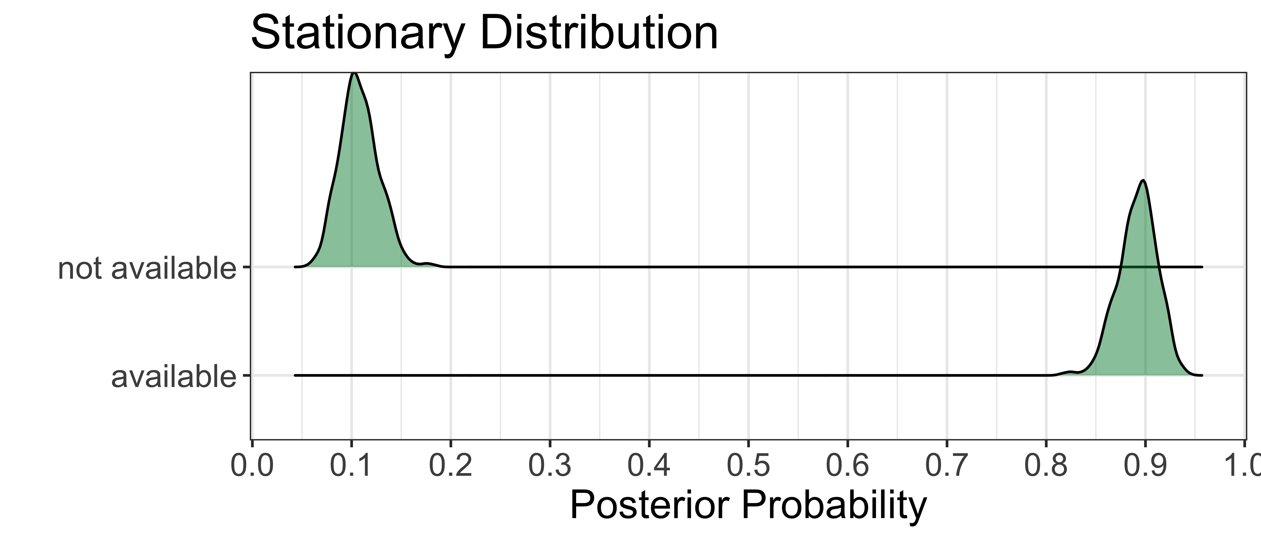
What about competition weeks? The table below summarizes the results for the observation model, where the probability of competing in a given week is given for each latent state. When a player is fit and available to play, the model suggests that they are expected to be competing for 2 of every 3 weeks, on average. A player that is not available, however, may still compete but it would be very unlikely, the posterior mean chance being just 3%. Importantly, neither probability is close to the boundary of 50% that we set in the priors, which tells us that we are identifying the conditional probabilities while not biasing their actual fit.
| Latent State | Posterior Mean | 95% Credible Interval |
|---|---|---|
| Available | 66 | 64 - 67 |
| Not available | 3 | 2 - 7 |
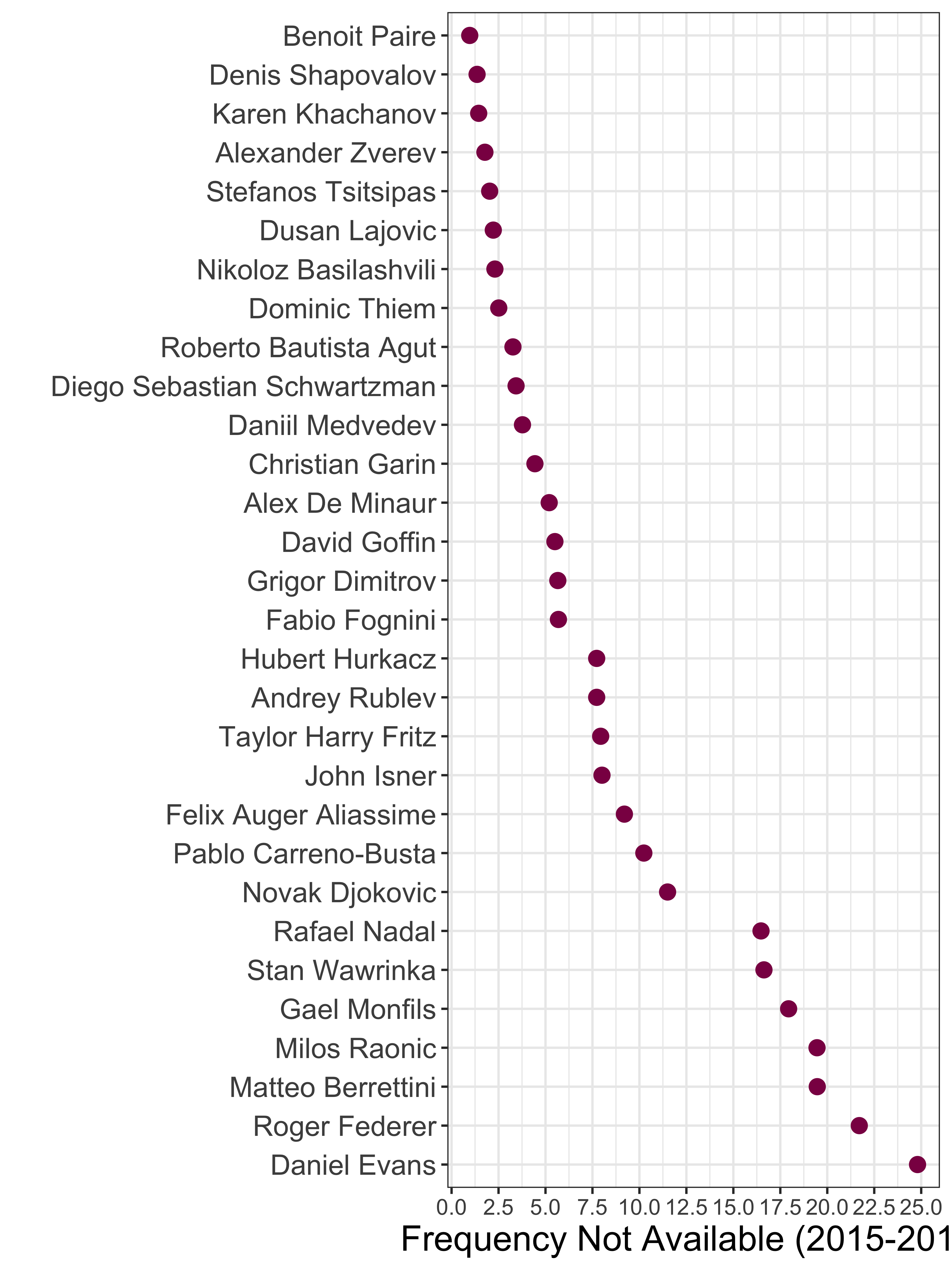
While these general properties are interesting, the real interest with this kind of model is what it can tell us about the situation of individual players. One question is which of the players in our sample of top 30 players have been the least available in recent years? The chart to the right shows the overall estimated frequency of time in the ‘not available’ latent state for each player. The majority of players are consistent with the steady state probability and are estimated to have been available 90% of the time or more. There are seven players who deviate from this pattern and were not available between 15% to 25% of the 2015 - 2019 period.
We can get a better idea of where those mean summaries came from by looking at the week-to-week estimated availability for the players with the most time in the ‘not available’ state. In the heatmaps below, the grey regions are the periods with the highest probability of a player not being available. The periods of injury and selective scheduling for Roger Federer, Rafael Nadal, Novak Djokovic and Stan Wawrinka are well known to us. And no one is likely to be surprised by the repeated absences of Milos Raonic, who has struggled to be fully healthy for a complete season since he turned pro.
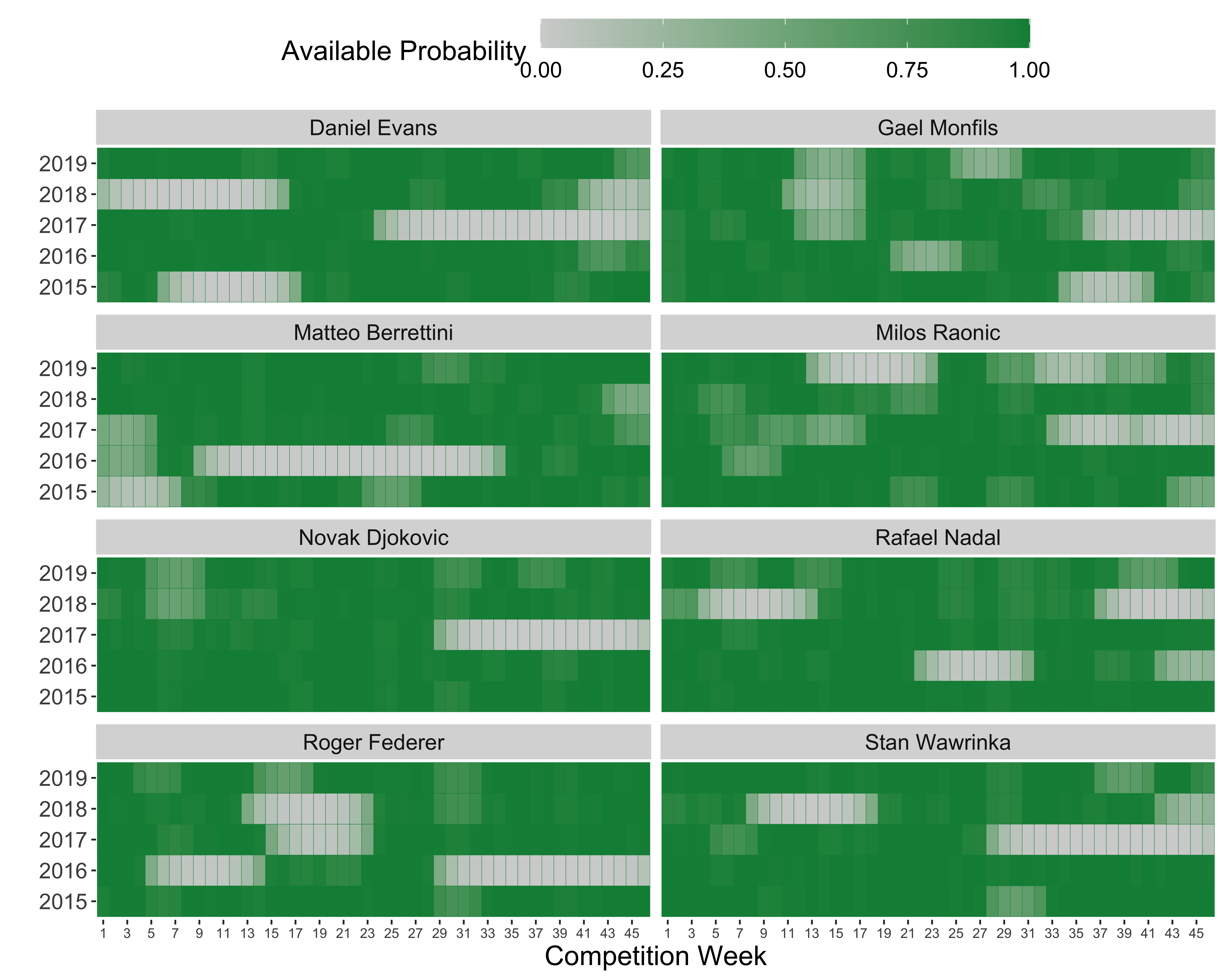
Many readers are likely to know that Dan Evans was forced out of competition for a time in 2017-2018 due to a drug suspension. The breaks for Gael Monfils and Matteo Berrettini would be the cases that most of us aren’t likely to have tracked as closely and would take a fair bit of googling to confirm. These examples alone make a strong case that even the most basic of availability models are giving us reasonable results and would already be a pretty useful tool for tracking the historical availability of players in an automated way.
Stan Availability Model
functions {
    matrix make_matrix(vector[] x, int d){
        matrix[d,d] X;

        for(i in 1:d)
            X[i] = x[i]';

    return X;
    }
}

data {
    int<lower=0> N;  // Player seasons
    int<lower=0> T; // Weeks
    int<lower=0> S; // Latent states
    matrix<lower=0,upper=1>[N,T] y; // Player x Observations
}

parameters {
    simplex[S] rho; // Initial state prob
    simplex[S] A[S]; // Transition matrix
    real theta0[S]; // Emission prob
}

transformed parameters {
    real<lower=0,upper=1> theta[S]; // Emission prob

    // Constraint
    theta[1] = 0.5 + (1 - 0.5) * inv_logit(theta0[1]); // Greater than 50%
    theta[2] = 0.5 * inv_logit(theta0[2]); // Less than 50%
}

model {
    matrix[S,T] yS[N]; // Hold log probabilities

    for(n in 1:N)
        for(s in 1:S)
            yS[n, s] = log(y[n] * theta[s] + (1 - y[n]) * (1 - theta[s]));

    for(s in 1:S)
        theta0[s] ~ std_normal();


    for(s in 1:S)
        A[s] ~ dirichlet(rep_vector(1., S));

     rho ~ dirichlet(rep_vector(1., S));

     for(n in 1:N)
         target += hmm_marginal(yS[n], make_matrix(A, S), rho);
}

generated quantities {
    int<lower=0,upper=S> latent_states[N,T];
    matrix<upper=0>[S,T] yS[N]; // Hold log probabilities

    for(n in 1:N)
        for(s in 1:S)
            yS[n, s] = log(y[n] * theta[s] + (1 - y[n]) * (1 - theta[s]));

    for(n in 1:N)
        latent_states[n] = hmm_latent_rng(yS[n], make_matrix(A, S), rho);
}